[1] "zh_CN.UTF-8/zh_CN.UTF-8/zh_CN.UTF-8/C/zh_CN.UTF-8/zh_CN.UTF-8"载入需要的程序包:sysfonts载入需要的程序包:showtextdb[1] "zh_CN.UTF-8/zh_CN.UTF-8/zh_CN.UTF-8/C/zh_CN.UTF-8/zh_CN.UTF-8"载入需要的程序包:sysfonts载入需要的程序包:showtextdb载入需要的程序包:haven载入需要的程序包:sjlabelled
载入程序包:'sjlabelled'The following objects are masked from 'package:haven':
as_factor, read_sas, read_spss, read_stata, write_sas, zap_labelsConverting atomic to factors. Please wait...载入需要的程序包:sjPlot| ID | Name | Label | Values | Value Labels |
|---|---|---|---|---|
| 1 | q69_1 | q69-1我对有益于国家社会的公共计划深感兴趣 | 1 2 3 4 5 6 |
1. 非常不同意 2. 不同意 3. 有点不同意 4. 有点同意 5. 同意 6. 非常同意 |
| 2 | q69_2 | q69_2看到他人能从公共计划中受益能带给我相当大的满足感 | 1 2 3 4 5 6 |
1. 非常不同意 2. 不同意 3. 有点不同意 4. 有点同意 5. 同意 6. 非常同意 |
| 3 | q69_3 | q69_3与他人分享自己对政策的观点对我而言是极有吸引力的事情 | 1 2 3 4 5 6 |
1. 非常不同意 2. 不同意 3. 有点不同意 4. 有点同意 5. 同意 6. 非常同意 |
| 4 | q69_4 | q69_4我认为公共服务是一种公民责任 | 1 2 3 4 5 6 |
1. 非常不同意 2. 不同意 3. 有点不同意 4. 有点同意 5. 同意 6. 非常同意 |
| 5 | q69_5 | q69_5有意义的公共服务对我很重要 | 1 2 3 4 5 6 |
1. 非常不同意 2. 不同意 3. 有点不同意 4. 有点同意 5. 同意 6. 非常同意 |
| 6 | q69_6 | q69_6为公共利益奋斗是我的职责 | 1 2 3 4 5 6 |
1. 非常不同意 2. 不同意 3. 有点不同意 4. 有点同意 5. 同意 6. 非常同意 |
| 7 | q69_7 | q69_7当我看到弱势的人受害总是感到于心不忍 | 1 2 3 4 5 6 |
1. 非常不同意 2. 不同意 3. 有点不同意 4. 有点同意 5. 同意 6. 非常同意 |
| 8 | q69_8 | q69_8我经常提醒自己,人们总是互相依赖的 | 1 2 3 4 5 6 |
1. 非常不同意 2. 不同意 3. 有点不同意 4. 有点同意 5. 同意 6. 非常同意 |
| 9 | q69_9 | q69_9当看到人们的悲惨或痛苦时我会感到难过 | 1 2 3 4 5 6 |
1. 非常不同意 2. 不同意 3. 有点不同意 4. 有点同意 5. 同意 6. 非常同意 |
| 10 | q69_10 | q69_10对人民、社会做出贡献,比我个人的生涯发展更有意义 | 1 2 3 4 5 6 |
1. 非常不同意 2. 不同意 3. 有点不同意 4. 有点同意 5. 同意 6. 非常同意 |
| 11 | q69_11 | q69_11只要我认为对大众有利,我愿意冒着失去陞迁机会的风险去争取 | 1 2 3 4 5 6 |
1. 非常不同意 2. 不同意 3. 有点不同意 4. 有点同意 5. 同意 6. 非常同意 |
| 12 | q69_12 | q69_12我认为大我之责任当在小我之前 | 1 2 3 4 5 6 |
1. 非常不同意 2. 不同意 3. 有点不同意 4. 有点同意 5. 同意 6. 非常同意 |
载入需要的程序包:psych vars n mean sd median trimmed mad min max range skew kurtosis
q69_1* 1 1113 4.37 0.96 4 4.39 1.48 1 6 5 -0.45 0.67
q69_2* 2 1113 4.55 0.90 5 4.57 1.48 1 6 5 -0.32 0.48
q69_3* 3 1113 4.16 1.08 4 4.17 1.48 1 6 5 -0.39 0.19
q69_4* 4 1113 4.57 0.88 5 4.57 1.48 1 6 5 -0.49 1.36
q69_5* 5 1113 4.60 0.90 5 4.62 1.48 1 6 5 -0.44 0.75
q69_6* 6 1113 4.25 0.96 4 4.26 1.48 1 6 5 -0.35 0.62
q69_7* 7 1113 4.68 0.90 5 4.71 1.48 1 6 5 -0.52 0.91
q69_8* 8 1113 4.47 0.93 4 4.50 1.48 1 6 5 -0.40 0.33
q69_9* 9 1113 4.75 0.84 5 4.76 1.48 1 6 5 -0.42 0.82
q69_10* 10 1113 4.02 1.10 4 4.01 1.48 1 6 5 -0.17 -0.04
q69_11* 11 1113 3.62 1.16 4 3.64 1.48 1 6 5 -0.11 -0.12
q69_12* 12 1113 3.80 1.11 4 3.84 1.48 1 6 5 -0.21 0.07
se
q69_1* 0.03
q69_2* 0.03
q69_3* 0.03
q69_4* 0.03
q69_5* 0.03
q69_6* 0.03
q69_7* 0.03
q69_8* 0.03
q69_9* 0.03
q69_10* 0.03
q69_11* 0.03
q69_12* 0.03 q69_1 q69_2 q69_3 q69_4 q69_5 q69_6 q69_7 q69_8
"factor" "factor" "factor" "factor" "factor" "factor" "factor" "factor"
q69_9 q69_10 q69_11 q69_12
"factor" "factor" "factor" "factor" q69_1 q69_2 q69_3 q69_4 q69_5 q69_6 q69_7 q69_8
"numeric" "numeric" "numeric" "numeric" "numeric" "numeric" "numeric" "numeric"
q69_9 q69_10 q69_11 q69_12
"numeric" "numeric" "numeric" "numeric" MSA 针对单一变量
• < 0.50 → 不适合做因子分析,该变量通常建议删除
• 0.50 ≤ MSA < 0.60 → 勉强可以接受
• 0.60 ≤ MSA < 0.70 → 一般可接受
• 0.70 ≤ MSA < 0.80 → 良好
• 0.80 ≤ MSA < 0.90 → 非常好
• MSA ≥ 0.90 → 极佳
1.当所有变量的「简单相关系数」大于「偏相关系数平方和」时,KMO愈接近1,表示变量间的相关性愈强,原有变量愈适合做因素分析。一般采用Kalser标准,> 0.7以上,即表示有特定的因素存在可供萃取,成为变项的共同因素,适合作因素分析。
2.当所有变量的「简单相关系数平方和」接近0时,KMO愈接近0,表示变量间的相关性愈弱,原有变量愈不适合做因素分析。
KMO 针对整体
• < 0.50 不适合,通常不建议做因子分析
• 0.50–0.59 不太适合,建议修正或删题
• 0.60–0.69 勉强适合,需谨慎
• 0.70–0.79 一般,仍可接受
• 0.80–0.89 良好,适合因子分析
• ≥ 0.90 极佳,非常适合因子分析
当Bartlett’s球形检验卡方值对应的p值 < 0.05时, 表示数据呈球形分布,各个变量在一定程度上相互独立,变项间有共同因素存在,适合进行因素分析。
| Component 1 | Component 2 | Component 3 | MSA | |
|---|---|---|---|---|
| q69-1我对有益于国家社会的公共计划深感兴趣 | 0.84 | -0.16 | -0.19 | 0.90 |
| q69_2看到他人能从公共计划中受益能带给我相当大的满足感 | 0.83 | -0.26 | -0.15 | 0.90 |
| q69_3与他人分享自己对政策的观点对我而言是极有吸引力的事情 | 0.79 | -0.10 | -0.23 | 0.96 |
| q69_4我认为公共服务是一种公民责任 | 0.74 | -0.30 | -0.28 | 0.94 |
| q69_5有意义的公共服务对我很重要 | 0.74 | -0.34 | -0.26 | 0.94 |
| q69_6为公共利益奋斗是我的职责 | 0.66 | -0.30 | -0.45 | 0.95 |
| q69_7当我看到弱势的人受害总是感到于心不忍 | 0.21 | -0.83 | -0.21 | 0.87 |
| q69_8我经常提醒自己,人们总是互相依赖的 | 0.26 | -0.66 | -0.21 | 0.95 |
| q69_9当看到人们的悲惨或痛苦时我会感到难过 | 0.22 | -0.86 | -0.15 | 0.86 |
| q69_10对人民、社会做出贡献,比我个人的生涯发展更有意义 | 0.31 | -0.35 | -0.73 | 0.94 |
| q69_11只要我认为对大众有利,我愿意冒着失去陞迁机会的风险去争取 | 0.27 | -0.13 | -0.86 | 0.87 |
| q69_12我认为大我之责任当在小我之前 | 0.23 | -0.20 | -0.86 | 0.88 |
| Proportion of Variance | 54.73 % | 10.39 % | 9.53 % | |
| Cumulative Proportion | 54.73 % | 65.12 % | 74.65 % | |
| Cronbach's α | 0.92 | 0.80 | 0.88 | |
| Kaiser-Meyer-Olkin | 0.92 | |||
| varimax-rotation | ||||
$chisq
[1] 8983.454

$p.value
[1] 0

$df
[1] 66
sjPlot::tab_pca() 会呈现转轴后的factor loading及各因素测量题项的Cronbach's α
结果:
每个题目的MSA都在0.8以上,最小的MSA为0.86
KMO=0.92
Bartlett 球形度检定的\(卡方值=8983.454, df=66, P=0.00\)
上述结果告诉我们一个事实,这个问卷题项所得的测量结果,非常适合进行因子分析。
因子的萃取,采用主成份分析法(PCA)+最大变异转轴法(Varimax Rotation),基本目的是为了获得因子对于变量(问卷题项)的最大解释变异,且假设因子之间没有相关性。
载入需要的程序包:performance# Is the data suitable for Factor Analysis?
- Sphericity: Bartlett's test of sphericity suggests that there is sufficient significant correlation in the data for factor analysis (Chisq(66) = 8983.45, p < .001).
- KMO: The Kaiser, Meyer, Olkin (KMO) overall measure of sampling adequacy suggests that data seems appropriate for factor analysis (KMO = 0.92). The individual KMO scores are: q69_1 (0.90), q69_2 (0.90), q69_3 (0.96), q69_4 (0.94), q69_5 (0.94), q69_6 (0.95), q69_7 (0.87), q69_8 (0.95), q69_9 (0.86), q69_10 (0.94), q69_11 (0.87), q69_12 (0.88).载入需要的程序包:parameters载入需要的程序包:nFactors# Method Agreement Procedure:
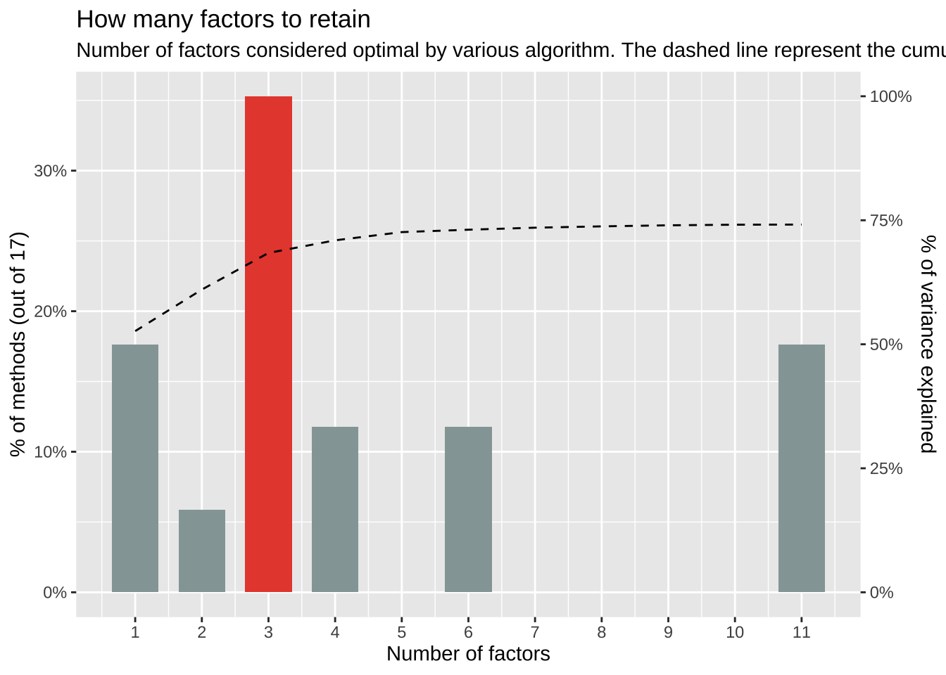
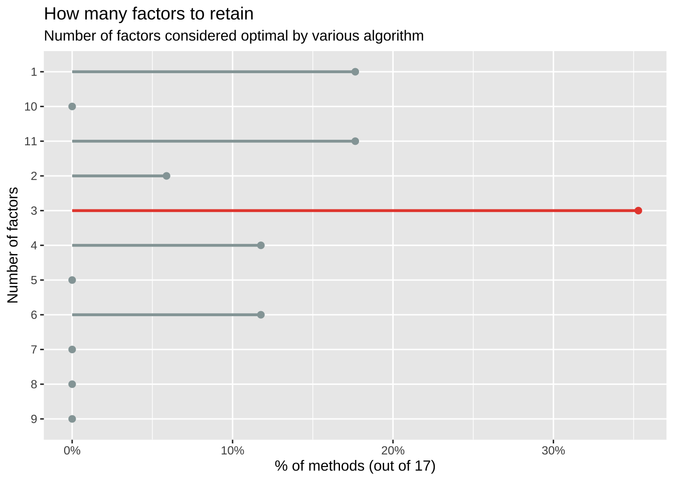
The choice of 3 dimensions is supported by 6 (35.29%) methods out of 17 (CNG, Parallel analysis, Kaiser criterion, Scree (SE), Scree (R2), Velicer's MAP).结果显示: 在17种运算方法中,大约有6种方法(35.29%),建议萃取3个因素。
透过转轴后的因子矩阵,将题项进行因子萃取, 并透过直交转轴Varimax最大变异法,产生一个 “转轴后的因子矩阵” (Rotated Component Matrix),如 图 1 所示:
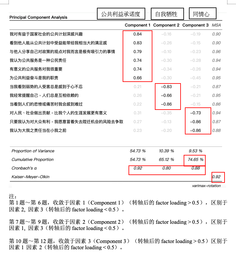
表格中的数字,代表「转轴后的因子负荷量」(Rotated factor loading),表示测量题项与因子之间的相关。loading数值愈高,代表该测量题项愈能代表该因素,「转轴后因子负荷量的平方」约略等于「因子」对于各题解释变异量的估计 (Hair 等, 1998)
从 图 1 可以看到:
第1题~第6题,收敛于因素1(Component 1)(Rotated factor loading > 0.5),区别于因素2, 因素3(转轴后的factor loading < 0.5)。
第7题~第9题,收敛于因素2(Component 2)(Rotated factor loading > 0.5),区别于因素1, 因素3(转轴后的factor loading < 0.5)。
第10题~第12题,收敛于因素3(Component 3)(Rotated factor loading > 0.5)区别于因素1, 因素2(转轴后的factor loading < 0.5)。
也就是说,这12道题目的测量,符合了收敛效度与区别效度。
Principal Components Analysis
Call: principal(r = r, nfactors = nfactors, residuals = residuals,
    rotate = rotate, n.obs = n.obs, covar = covar, scores = scores,
    missing = missing, impute = impute, oblique.scores = oblique.scores,
    method = method, use = use, cor = cor, correct = 0.5, weight = NULL)
Standardized loadings (pattern matrix) based upon correlation matrix
        RC1  RC3  RC2   h2   u2 com
q69_1  0.84 0.19 0.16 0.76 0.24 1.2
q69_2  0.83 0.15 0.26 0.78 0.22 1.3
q69_3  0.79 0.23 0.10 0.69 0.31 1.2
q69_4  0.74 0.28 0.30 0.72 0.28 1.6
q69_5  0.74 0.26 0.34 0.73 0.27 1.7
q69_6  0.66 0.45 0.30 0.72 0.28 2.2
q69_7  0.21 0.21 0.83 0.78 0.22 1.3
q69_8  0.26 0.21 0.66 0.55 0.45 1.5
q69_9  0.22 0.15 0.86 0.81 0.19 1.2
q69_10 0.31 0.73 0.35 0.76 0.24 1.8
q69_11 0.27 0.86 0.13 0.83 0.17 1.2
q69_12 0.23 0.86 0.20 0.84 0.16 1.2

                       RC1  RC3  RC2
SS loadings           3.92 2.59 2.44
Proportion Var        0.33 0.22 0.20
Cumulative Var        0.33 0.54 0.75
Proportion Explained  0.44 0.29 0.27
Cumulative Proportion 0.44 0.73 1.00

Mean item complexity =  1.5
Test of the hypothesis that 3 components are sufficient.

The root mean square of the residuals (RMSR) is  0.04
 with the empirical chi square  191.62  with prob <  2.9e-24

Fit based upon off diagonal values = 1# Rotated loadings from Principal Component Analysis (varimax-rotation)
Variable | RC1 | RC3 | RC2 | Complexity | Uniqueness
-------------------------------------------------------
q69_1 | 0.84 | 0.19 | 0.16 | 1.18 | 0.24
q69_2 | 0.83 | 0.15 | 0.26 | 1.26 | 0.22
q69_3 | 0.79 | 0.23 | 0.10 | 1.20 | 0.31
q69_4 | 0.74 | 0.28 | 0.30 | 1.63 | 0.28
q69_5 | 0.74 | 0.26 | 0.34 | 1.67 | 0.27
q69_6 | 0.66 | 0.45 | 0.30 | 2.23 | 0.28
q69_7 | 0.21 | 0.21 | 0.83 | 1.26 | 0.22
q69_8 | 0.26 | 0.21 | 0.66 | 1.50 | 0.45
q69_9 | 0.22 | 0.15 | 0.86 | 1.19 | 0.19
q69_10 | 0.31 | 0.73 | 0.35 | 1.83 | 0.24
q69_11 | 0.27 | 0.86 | 0.13 | 1.24 | 0.17
q69_12 | 0.23 | 0.86 | 0.20 | 1.25 | 0.16
The 3 principal components (varimax rotation) accounted for 74.65% of the total variance of the original data (RC1 = 32.68%, RC3 = 21.62%, RC2 = 20.35%).Complexity(复杂度)
定义:一个题项在多个因子上都有显著载荷时,复杂度就高。
解释:
    ▪︎ 接近 1 → 题项主要由单一因子解释,结构清晰。

    ▪︎ 大于 1 → 题项同时受多个因子影响,解释较复杂。
用途:帮助判断题项是否「跨因子」,是否需要重新设计或删除。
• Uniqueness(独特性 / 特有性)
定义:题项的变异中,未被任何因子解释的比例。
解释:
    ▪︎ 接近 0 → 题项大部分变异被因子解释,适合保留。

    ▪︎ 接近 1 → 题项几乎没有被因子解释,可能不适合。
用途:判断题项是否与因子结构契合。
实务建议:
• Complexity:理想值接近1,表示题项只对单一因子有明显贡献。若 >1.5,可能需要检查题项是否跨因子。
• Uniqueness: <0.5,表示题项至少有一半以上的变异能被因子解释。若 >0.7,通常考虑删除或修正。
因子的命名,可以因子与题项间最高的 “Rotated factor loading”为参考依据。
因素一:公共利益承诺度(Commitment to the public interest)
因素二:自我牺牲(self-sacrifice)
因素三:同情心(compassion)
载入需要的程序包:lavaanThis is lavaan 0.6-21
lavaan is FREE software! Please report any bugs.
载入程序包:'lavaan'The following object is masked from 'package:psych':
cor2cov载入需要的程序包:semTools ###############################################################################This is semTools 0.5-8All users of R (or SEM) are invited to submit functions or ideas for functions.###############################################################################
载入程序包:'semTools'The following object is masked from 'package:parameters':
kurtosisThe following objects are masked from 'package:psych':
reliability, skew检验标准:(Fornell & Larcker, 1981)
–每个构念(因子)的 CR (Composite Reliability)(组合信度) > 0.7
–每个构念(因子)的 AVE (Average Variance Extracted)(平均方差萃取量) 应 > 0.5
$fac_1

Composite `fac_1` is composed of observed variables:
    q69_1, q69_2, q69_3, q69_4, q69_5, q69_6
True-score variance is represented by common factor(s):
    fac_1
Total variance of composite `fac_1` determined from the unrestricted model.
The proportion attributable to "true" scores is its model-based estimate of reliability ("omega"):

[1] 0.916

$fac_2

Composite `fac_2` is composed of observed variables:
    q69_7, q69_8, q69_9
True-score variance is represented by common factor(s):
    fac_2
Total variance of composite `fac_2` determined from the unrestricted model.
The proportion attributable to "true" scores is its model-based estimate of reliability ("omega"):

[1] 0.815

$fac_3

Composite `fac_3` is composed of observed variables:
    q69_10, q69_11, q69_12
True-score variance is represented by common factor(s):
    fac_3
Total variance of composite `fac_3` determined from the unrestricted model.
The proportion attributable to "true" scores is its model-based estimate of reliability ("omega"):

[1] 0.881fac_1 fac_2 fac_3
0.651 0.587 0.708 我们得到:
fac_1 的 CR (即 “omega”)=0.916
fac_2 的 CR (即 “omega”)=0.815
fac_3 的 CR (即 “omega”)=0.881
fac_1 的 AVE =0.651
fac_2 的 AVE =0.587
fac_3 的 AVE =0.708
检验标准:(Fornell & Larcker, 1981)
–每个构念(因子)的 sqrt_AV (AVE平方根) 应 > 其与其他构念(因子)的 cor_matrix( 相关系数矩阵)
fac_1 fac_2 fac_3
0.807 0.766 0.841 fac_1 fac_2 fac_3
fac_1 1.000
fac_2 0.643 1.000
fac_3 0.682 0.569 1.000分析结果:
问卷题项量表,每个构念(因子)的 “AVE平方根” 皆大于其与其他构念(因子)的 “相关系数” 。如 表 1 所示。
因此,问卷题项量表在各个构念(因子)之间具备了区别效度。
| FAC_1 | FAC_2 | FAC_3 | |
|---|---|---|---|
| FAC_1 | 0.807 |
||
| FAC_2 | 0.643 | 0.766 |
|
| FAC_3 | 0.682 | 0.569 | 0.841 |
注:
1. 对角线数值为 “构念(因子)的AVE平方根”(sqrt_AVE)
2. 不同FAC因子之间的数值(例如:FAC_1 vs. FAC_2),为 “构念(因子)与其构念(因子)间的 “相关系数”
我们可以将前述的 CR, AVE, 与 表 1 合并放在一个表,一览验证性因子分析(CFA)方法下的收敛效度与区别效度。如:表 2 所示。
| 收敛效度 | 区别效度 | ||||
| CR(>0.7) | AVE(0.5) | FAC_1 | FAC_2 | FAC_3 | |
| FAC_1 | 0.916 | 0.651 | 0.807 |
||
| FAC_2 | 0.815 | 0.587 | 0.643 | 0.766 |
|
| FAC_3 | 0.881 | 0.708 | 0.682 | 0.569 | 0.841 |
注:
1. 划底线的数值为 “构念(因子)的AVE平方根”(sqrt_AVE)
2. 不同FAC因子之间的数值(例如:FAC_1 vs. FAC_2),为 “构念(因子)与其构念(因子)间的 “相关系数”
Cronbach’s α 的公式如下:
\[\alpha= \frac{k}{k-1} \left(1 - \frac{\sum_{i=1}^{k} sigma^2_{Y_i}}{\sigma^2_{X}}\right)\]
其中:
\(k\):题项数
\(sigma^2_{Y_i}\):第 \(i\) 题的变异数
\(sigma^2_{X}\):总分的变异数
[1] 0.9181484# Item Reliability
Item | Alpha if deleted | Total Correlation | Discrimination
-------------------------------------------------------------
q69_1 | 0.90 | 0.85 | 0.78
q69_2 | 0.90 | 0.86 | 0.80
q69_3 | 0.91 | 0.82 | 0.72
q69_4 | 0.90 | 0.85 | 0.78
q69_5 | 0.90 | 0.86 | 0.79
q69_6 | 0.91 | 0.84 | 0.76
Mean inter-item-correlation = 0.658 Cronbach's alpha = 0.918结果:
总的Cronbach’s alpha=0.92
呈现如果删除某一个item(变量), 总的Cronbach’s alpha会变成多少?(作为删除题目参考)。结果显示,没什么题目需要删除的(信度都很高)。
[1] 0.7955305# Item Reliability
Item | Alpha if deleted | Total Correlation | Discrimination
-------------------------------------------------------------
q69_7 | 0.67 | 0.87 | 0.68
q69_8 | 0.84 | 0.79 | 0.53
q69_9 | 0.65 | 0.87 | 0.71
Mean inter-item-correlation = 0.569 Cronbach's alpha = 0.796结果:
总的Cronbach’s alpha=0.80
如果删除q69_8,Cronbach’s alpha会提高到0.84
[1] 0.8762228# Item Reliability
Item | Alpha if deleted | Total Correlation | Discrimination
--------------------------------------------------------------
q69_10 | 0.86 | 0.87 | 0.72
q69_11 | 0.81 | 0.91 | 0.78
q69_12 | 0.80 | 0.91 | 0.79
Mean inter-item-correlation = 0.702 Cronbach's alpha = 0.876结果:
总的Cronbach’s alpha=0.88
如果删除q69_10,Cronbach’s alpha会提高到0.86
最后,我们可以将前述使用 EFA 与 CFA 因子分析的问卷题目信效度结果,统整理如 表 3
以下代码整合 Cronbach’s α、组合信度(CR)、AVE、√AVE 与因子间相关系数,生成完整的论文报告表。
载入程序包:'dplyr'The following object is masked from 'package:kableExtra':
group_rowsThe following object is masked from 'package:sjlabelled':
as_labelThe following objects are masked from 'package:stats':
filter, lagThe following objects are masked from 'package:base':
intersect, setdiff, setequal, union# 1. 提取因子-题目对应关系
factor_items <- lavInspect(fit, "list") |>
as.data.frame() |>
dplyr::filter(op == "=~") |>
dplyr::select(lhs, rhs)
factor_names <- unique(factor_items$lhs)
n_f <- length(factor_names)
# 2. 旋转因子载荷(RC1=fac_1, RC2=fac_2, RC3=fac_3,重排对齐因子顺序)
lm_raw <- unclass(pca$loadings)
lm_ordered <- lm_raw[, c("RC1", "RC2", "RC3")]
colnames(lm_ordered) <- c("F1", "F2", "F3")
lm_disp <- as.data.frame(lapply(as.data.frame(round(lm_ordered, 3)), function(x) {
ifelse(abs(x) < 0.5, "", sprintf("%.3f", x))
}))
rownames(lm_disp) <- rownames(lm_ordered)
# 3. 信效度指标
alpha_vals <- sapply(factor_names, function(f) {
items <- factor_items$rhs[factor_items$lhs == f]
psych::alpha(mydata[, items])$total$raw_alpha
})
ave_vals <- AVE(fit)
cr_vals_num <- sapply(compRelSEM(fit), as.numeric)
# 4. 因子-题目对应与中文名称
fac_map <- list(
fac_1 = paste0("q69_", 1:6),
fac_2 = paste0("q69_", 7:9),
fac_3 = paste0("q69_", 10:12)
)
fac_labels <- c(
fac_1 = "F1 公共利益",
fac_2 = "F2 自我牺牲",
fac_3 = "F3 同情心"
)
# 5. 因子相关矩阵
cor_mat <- lavInspect(fit, "cor.lv")
# 6. 构建整合大表(题目行 + 每因子汇总行,汇总行含区别效度)
rows <- list()
for (k in seq_along(factor_names)) {
fname <- factor_names[k]
items <- fac_map[[fname]]
# 题目行
for (item in items) {
rows[[length(rows) + 1]] <- c(
item,
lm_disp[item, "F1"], lm_disp[item, "F2"], lm_disp[item, "F3"],
"", "", "", ""
)
}
# 汇总行:F1/F2/F3 填判别效度(对角线 = √AVE,非对角线 = 因子相关 r)
disc_vals <- sapply(seq_along(factor_names), function(j) {
if (j == k) paste0("(", sprintf("%.3f", sqrt(ave_vals[k])), ")")
else sprintf("%.3f", cor_mat[k, j])
})
rows[[length(rows) + 1]] <- c(
paste0(fac_labels[fname], " 汇总(区别效度)"),
disc_vals[1], disc_vals[2], disc_vals[3],
sprintf("%.3f", alpha_vals[k]),
sprintf("%.3f", cr_vals_num[k]),
sprintf("%.3f", ave_vals[k]),
sprintf("%.3f", sqrt(ave_vals[k]))
)
}
big_table <- as.data.frame(do.call(rbind, rows), stringsAsFactors = FALSE)
colnames(big_table) <- c("题目", "F1", "F2", "F3", "α", "CR", "AVE", "√AVE")
summary_rows <- which(grepl("汇总(区别效度)", big_table$题目))
# 7. 输出 HTML 表格
kable(big_table,
format = "html",
align = c("l", rep("c", 7)),
escape = FALSE) |>
kable_styling(
bootstrap_options = c("striped", "hover", "bordered"),
full_width = FALSE,
font_size = 13
) |>
add_header_above(c(
" " = 1,
"EFA视角下的旋转因子载荷(收敛效度) 与区别效度" = 3,
"信度" = 1,
"CFA视角下的收敛效度与区别效度" = 3
)) |>
row_spec(summary_rows, bold = TRUE, italic = TRUE,
background = "#e8e8e8", color = "#1a5276") |>
pack_rows("因子一(公共利益承诺度)", 1, 7) |>
pack_rows("因子二(自我牺牲)", 8, 11) |>
pack_rows("因子三(同情心)", 12, 15) |>
kableExtra::footnote(
general = paste0(
"旋转方法:主成分分析(Varimax 旋转);载荷绝对值 < 0.5 不显示。",
"汇总行的 F1/F2/F3 为区别效度矩阵:括号内为 √AVE(对角线),",
"其余为因子间相关系数 r;√AVE > r 表示区别效度良好。",
"α = Cronbach's α;CR > 0.7、AVE > 0.5 表示收敛效度良好。"
),
general_title = "注:",
escape = FALSE
) |>
# 让脚注文字跨越所有列(kableExtra HTML 默认只占 1 列)
gsub(
pattern = 'colspan="1"><em>注',
replacement = paste0('colspan="', ncol(big_table), '"><em>注'),
x = _
) |>
structure(class = "knitr_kable", format = "html")| 题目 | F1 | F2 | F3 | α | CR | AVE | √AVE |
|---|---|---|---|---|---|---|---|
| 因子一(公共利益承诺度) | |||||||
| q69_1 | 0.836 | ||||||
| q69_2 | 0.830 | ||||||
| q69_3 | 0.793 | ||||||
| q69_4 | 0.739 | ||||||
| q69_5 | 0.742 | ||||||
| q69_6 | 0.656 | ||||||
| F1 公共利益 汇总(区别效度) | (0.807) | 0.643 | 0.682 | 0.918 | 0.916 | 0.651 | 0.807 |
| 因子二(自我牺牲) | |||||||
| q69_7 | 0.830 | ||||||
| q69_8 | 0.664 | ||||||
| q69_9 | 0.859 | ||||||
| F2 自我牺牲 汇总(区别效度) | 0.643 | (0.766) | 0.569 | 0.796 | 0.815 | 0.587 | 0.766 |
| 因子三(同情心) | |||||||
| q69_10 | 0.733 | ||||||
| q69_11 | 0.863 | ||||||
| q69_12 | 0.865 | ||||||
| F3 同情心 汇总(区别效度) | 0.682 | 0.569 | (0.841) | 0.876 | 0.881 | 0.708 | 0.841 |
| 注: | |||||||
| 旋转方法:主成分分析(Varimax 旋转);载荷绝对值 < 0.5 不显示。汇总行的 F1/F2/F3 为区别效度矩阵:括号内为 √AVE(对角线),其余为因子间相关系数 r;√AVE > r 表示区别效度良好。α = Cronbach's α;CR > 0.7、AVE > 0.5 表示收敛效度良好。 | |||||||
以下使用 flextable 重建同一张表,可在渲染为 Word(.docx)时完整保留样式。
载入程序包:'flextable'The following objects are masked from 'package:kableExtra':
as_image, footnotelibrary(officer)
border_thick <- fp_border(color = "black", width = 1.5)
border_thin <- fp_border(color = "grey70", width = 0.5)
flextable(big_table) |>
set_header_labels(
题目 = "题目",
F1 = "F1", F2 = "F2", F3 = "F3",
α = "α", CR = "CR", AVE = "AVE", `√AVE` = "√AVE"
) |>
add_header_row(
values = c("", "EFA视角下的旋转因子载荷(收敛效度) 与区别效度", "信度", "CFA视角下的收敛效度与区别效度"),
colwidths = c(1, 3, 1, 3)
) |>
align(align = "center", part = "all") |>
align(j = 1, align = "left", part = "body") |>
bold(i = summary_rows, part = "body") |>
italic(i = summary_rows, part = "body") |>
color(i = summary_rows, color = "#1a5276", part = "body") |>
bg(i = summary_rows, bg = "#e8e8e8", part = "body") |>
hline(i = c(7, 11), border = border_thick, part = "body") |>
add_footer_lines(paste0(
"注:旋转方法:主成分分析(Varimax 旋转);载荷绝对值 < 0.5 不显示。",
"汇总行的 F1/F2/F3 为区别效度矩阵:括号内为 √AVE(对角线),",
"其余为因子间相关系数 r;√AVE > r 表示区别效度良好。",
"α = Cronbach's α;CR > 0.7、AVE > 0.5 表示收敛效度良好。"
)) |>
align(align = "left", part = "footer") |>
italic(part = "footer") |>
fontsize(size = 9, part = "footer") |>
border_outer(border = border_thick) |>
border_inner_h(border = border_thin, part = "body") |>
hline_top(border = border_thick, part = "header") |>
hline_bottom(border = border_thick, part = "header") |>
font(fontname = "Times New Roman", part = "all") |>
fontsize(size = 10, part = "all") |>
fontsize(size = 11, part = "header") |>
bold(part = "header") |>
autofit()EFA视角下的旋转因子载荷(收敛效度) 与区别效度 | 信度 | CFA视角下的收敛效度与区别效度 | |||||
|---|---|---|---|---|---|---|---|
题目 | F1 | F2 | F3 | α | CR | AVE | √AVE |
q69_1 | 0.836 | ||||||
q69_2 | 0.830 | ||||||
q69_3 | 0.793 | ||||||
q69_4 | 0.739 | ||||||
q69_5 | 0.742 | ||||||
q69_6 | 0.656 | ||||||
F1 公共利益 汇总(区别效度) | (0.807) | 0.643 | 0.682 | 0.918 | 0.916 | 0.651 | 0.807 |
q69_7 | 0.830 | ||||||
q69_8 | 0.664 | ||||||
q69_9 | 0.859 | ||||||
F2 自我牺牲 汇总(区别效度) | 0.643 | (0.766) | 0.569 | 0.796 | 0.815 | 0.587 | 0.766 |
q69_10 | 0.733 | ||||||
q69_11 | 0.863 | ||||||
q69_12 | 0.865 | ||||||
F3 同情心 汇总(区别效度) | 0.682 | 0.569 | (0.841) | 0.876 | 0.881 | 0.708 | 0.841 |
注:旋转方法:主成分分析(Varimax 旋转);载荷绝对值 < 0.5 不显示。汇总行的 F1/F2/F3 为区别效度矩阵:括号内为 √AVE(对角线),其余为因子间相关系数 r;√AVE > r 表示区别效度良好。α = Cronbach's α;CR > 0.7、AVE > 0.5 表示收敛效度良好。 | |||||||